Review: empirical asset pricing via machine learning

For a long time machine learning has been used in the financial industry, especially in the empirical asset pricing field. This paper conducts a comparative analysis among different machine learning methods, sets the lower bar for the out of sample predicting power of each methods. Since its publication, it already has more than 1000 citations and has become the benchmark for machine learning research.

Gu, Kelly, Xiu

1. Methodology

• statistic model
• objective function (minimize MSE)
• regularization

The general form of asset’s excess return -> an additive prediction error model:

where:

Assume: A balaced panel of stocks

1.1 Sample splitting and tuning via validation

Internet Apenddix D: (West, 2006)

• fixed scheme -> splits the data into training, validation, and testing samples. It estimates the model once from the training and validation samples, and attempts to fit all points in the testing sample using this fixed model estimate.
• rolling scheme -> splits the training and validation samples gradually shift forward in time to include more recent data, but holds the total number of time periods in each training and validation sample fixed.
• “recursive” performance evaluation scheme -> Like the rolling approach, it gradually includes more recent observations in the training and validation windows. But the recursive scheme always retains the entire history in the training sample, thus its window size gradually increases.

This paper they increase the training sample by a year, while maintaining a fixed size rolling sample for validation. They choose to not cross-validate in order to maintain the temporal ordering of the data for prediction.

1.2 Simple linear

The conditional expectations $g^\ast (\cdot)$ can be approximated by a linear function of the raw predictor variables and the parameter vector $\theta$.

The estimation of the simple linear model uses a standard least squares, or $l_2$, objective function is: \(\tag{4} \mathbb l(\theta) = \frac{1}{NT} \sum^N_{i=1} \sum^T_{t=1} (r_{i,t+1} - g(z_{i,t}: \theta))^2\)

Extension: Robust objective functions -> replacing equation (4) with a weighted least squares objective:

• $w_{it}$ could be $\frac{1}{N}$, $N$ is the number of stocks.
• $w_{it}$ could be propotional to the equity market value of stocks. in favor of large stocks

Heavy tails are a well-known attribut of returns. It will affect OLS estimation for its emphasis on large errors. To handle the outliers in machine learning, it is common to use Huber robust object function to counteract the deleterious effect of heavy-tailed observations, which is:

where \(H(x;\zeta) =\begin{cases} x^2, & if \ |x| \leq \zeta \\ 2\zeta|x|-\zeta^2, & if \ |x| > \zeta \end{cases}\)

1.3 Penalized linear

The difference is in the loss function:

In this paper they use Elastic Net, which is: \(\tag{8} \phi(\theta; \lambda, \rho) = \lambda(1-\rho) \sum^p_{j=1}|\theta_j| + \frac{1}{2}\lambda \rho \sum^p_{j=1}\theta^2_j\)

They use accelerated proximal gradient algorithm (Parikh and Boyd (2013) and Polson et al. (2015)) and accommodates both least squares and Huber objective functions. (In internet appendix B)

1.4 Dimension reduction: PCR and PLS

Rewrite equation (1)(2)(3) to vector form: \(\tag{9} R = Z\theta + E\)

Where $Z$ is $NT$ x $P$, $\Omega_K$ is $P$ x $K$, $\Theta_K$ is $K$ x $1$, $\tilde E$ is $NT$ x $1$

1.5 Generalized linear

Decompose model forcast error:

Generalized linear model make nonlinear transformation to original predictors as new additive terms in an otherwise linear model.

where $p(\cdot) = (p_1(\cdot), p_2(\cdot), …, p_k(\cdot))$, $\theta = (\theta_1, \theta_2, …, \theta_k)$ is now $K$ x $N$, they apply a spline series of order two: $(a, z, (z-c_1)^2, (z-c_2)^2, … , (z-c_{k-2})^2)$, where $c_1, c_2, …$ are knots.

Same with 1.2, they use OLS both with and without Huber robustness modification. Because the series expansion quickly mutilies the number of model parameters, they use the specialized penalization function for spline expansion setting which known as the group lasso:

1.6 Boosted regression trees and random forests

The model in equation (13) only captures the nonlinear effect, not the interactions among predictors. Expand the model to accomodate predictors’ intercations, the parameters expand accordingly. The generalized linear model become computationally infeasible. A popular aternaltive in machine learning is regression tree.

• K -> terminal nodes, ‘leaves’
• L -> depth

$ C_k(L)$ is one of the K partitions of the data, each partition is a product of up to L indicatior functions of the predictors. $\theta_k$ is a constant associated with partition k, it is the sample average of outcomes with the partition.

The basic idea is to myopically optimize forecast error at the start of each branch. At each new level, choose a sorting variable from the set of predictors and the split value to maximize the discrepancy among average outcomes in each bin. The loss associated with the forecast error for a branch C is call “Impurity”, which describes how similarly observations behave on either side of the split. The L2 impurity is used in this paper:

Tree model is the most prone to overfit among all models. Need to be heavily regularized:

• First regularization method is boosting: recursively combine many simple trees, the theory behind is that many weak learners may, as an ensemble, comprise a single “strong learner” with greater stability than a single complex tree. GBRT Gradien Boosted Regression Tree is used in this paper. With 3 tuning parameters L, V, B (L: depth of tree, v: shrinking factor $v\in(0,1)$, B: Number of trees)
• Second is using random forest. It is also a resemble method just like boosting. It draws B different bootstrap samples of the data, fits a separate regression tree to each, then average the forecasts. Random forest decorrelates trees using “dropout”, which considers only a randomly drawn subset of predictiors for splitting at each potential branch. Tuning parameters are tree depth(L), Number of predictors at each split, number of boostrap sample(B).

1.7 Neural networks

This paper use traditional ‘feed-forward’ networks, which consists one ‘input layer’, one or more ‘hidden layers’, and an ‘output layer’. Recent research shows that deeper networks can often achieve the same accuracy with fewer parameters. Meanwhile, for small dataset simple network with a few layers and nodes often perform better.

A deep neural network is challenging because:

• large number of parameters
• objective function is highly nonconvex
• recursive calculation (‘back propagation’ here) is prone to exploding or vanishing gradients.

The activation function used here is rectified linear unit (ReLU), which encourage sparsity in the number of active neurons and allows for faster derivative evaluation. \(\tag{17} x^{(l)}_k = ReLU \left(x^{(l-1)'} \theta^{(l-1)}_k \right)\)

High degree of nonlinearity, nonconvexity, and heavy parametrization in neural network force optimization highly computational intensive. To handle those issues stochastic gradient descent (SGD) is used to train a neural network.

Hence regulariztion of neural network needs more care. There are 5 regularization methods are used:

• L1 penalization of weighting parameters
• learning rate shrinkage (Kingma and Ba (2014))
• early stopping
• batch normalization (Loffe and Szegedy (2015))
• esemble

1.8 Performace evaluation

Out of sample r-squared

Remark: The denominntor of $R^2$ is the sum of squared excess returns without demeaning. The logical befind is that predictin future excess stock returns with historical averages underperforms a naive forecast of zero by a large margin, using historical mean will lower the bar for forecasting performance.

Use Diebold and Mariano (1995) test for pairwise comparisons of $R_2$ in different models: $DM_{12} = \bar d_{12}/\hat \delta_{\bar d_{12}}$ where

\(\tag{20} d_{12, t+1} = \frac{1}{n_{3,t+1}} \sum^{n_{3,t+1}}_ \left(\left(\hat e^{(1)}_{i,t+1} \right)^2 - \left(\hat e^{(2)}_{i,t+1}\right)^2 \right)\)

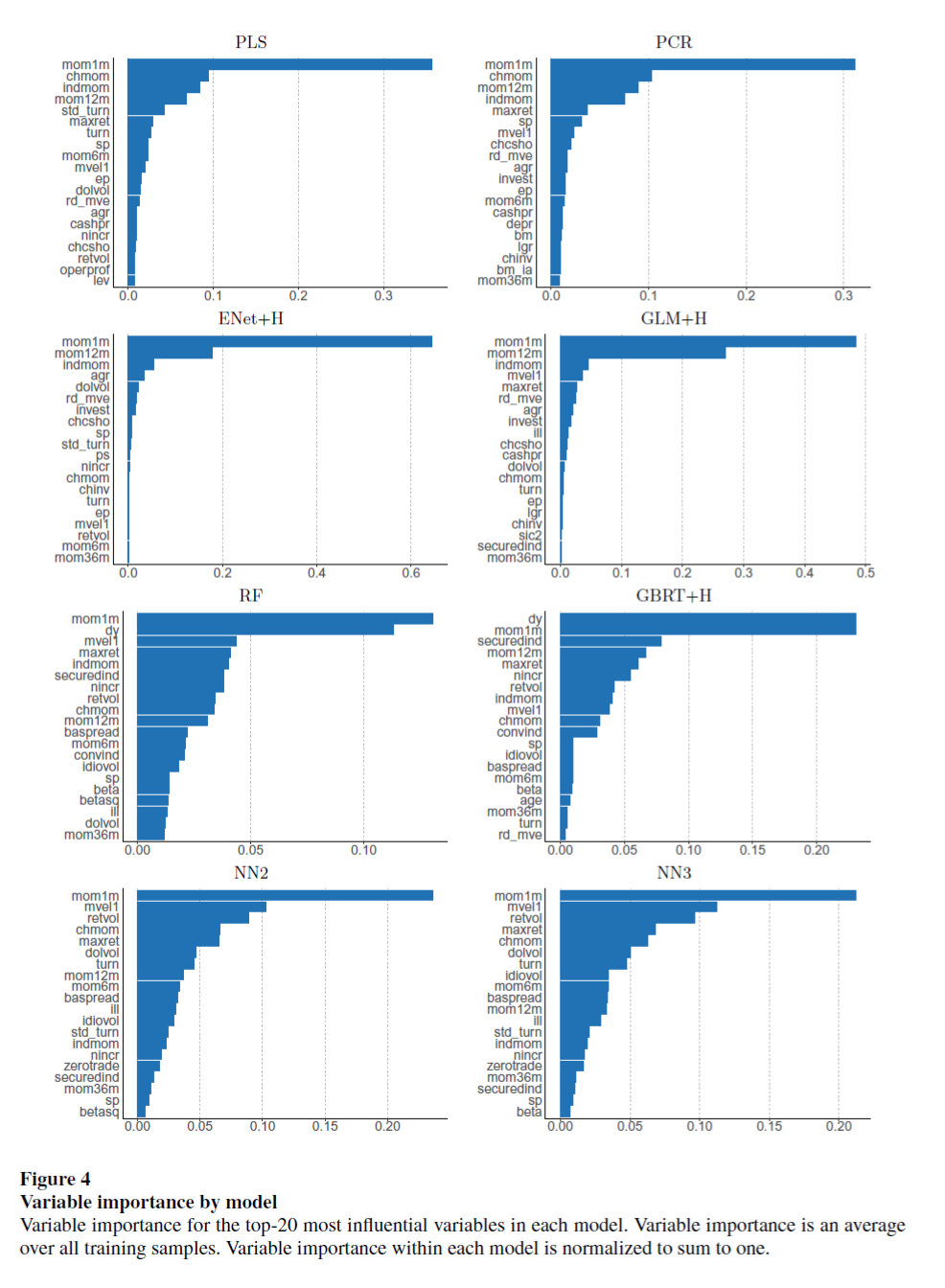
1.9 Variable importance and marginal relationships

$VI_j$ for the importance of the jth variable:

• Reduction in panel predictive $R^2$ from setting all values of predictor j to zero.
• Sum of squared partial derivatives (SSD).
• Trace out the marginal relationship between expected return and each characteristic.

2.1 Data and the overaching model

• U.S. monthly total individual equity listed in NYSE, AMEX, and NASDAQ from 1957-03 to 2016-12.
• Number of stocks more than 30,000.
• Stock level predictive characteristics 94.
• Macroeconomic predictors 8.
• Industry dummies 74.
• stock-level covariates $z_{i,t}$, in total 94x(8+1)+74=920

• Training sample 1957-1974 (18 years)
• Validation sample 1975-1986 (12 years)
• Testing sample 1987-2016 (30 years)
• The rolling window is 1 year instead of each month

2.2 The cross-section of individual stock

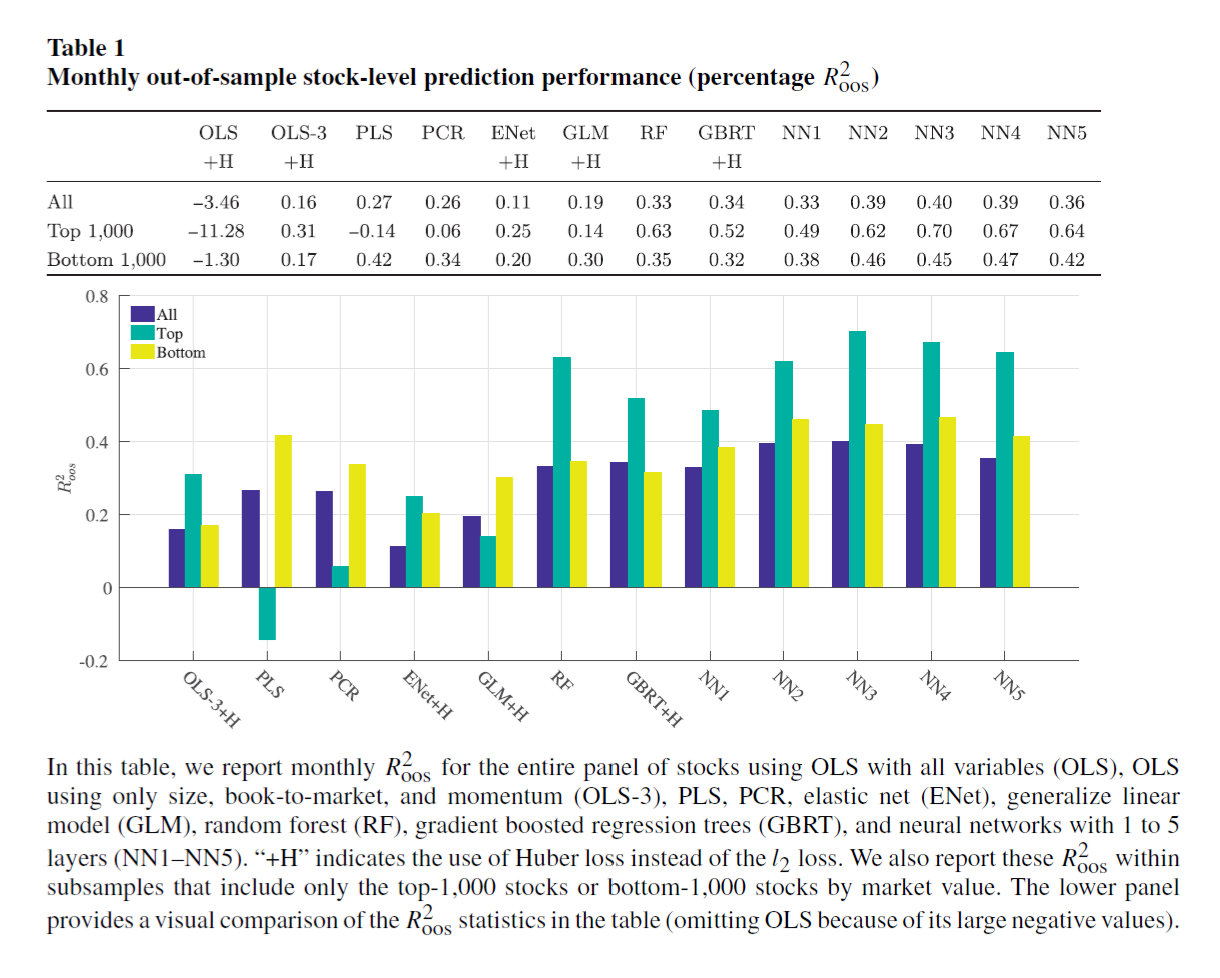
The out of sample $R^2$ of simple OLS model is negative, indicating that it is arbitrarily worse. The neural network with 3 layers has the best out of sample performance among all other models.

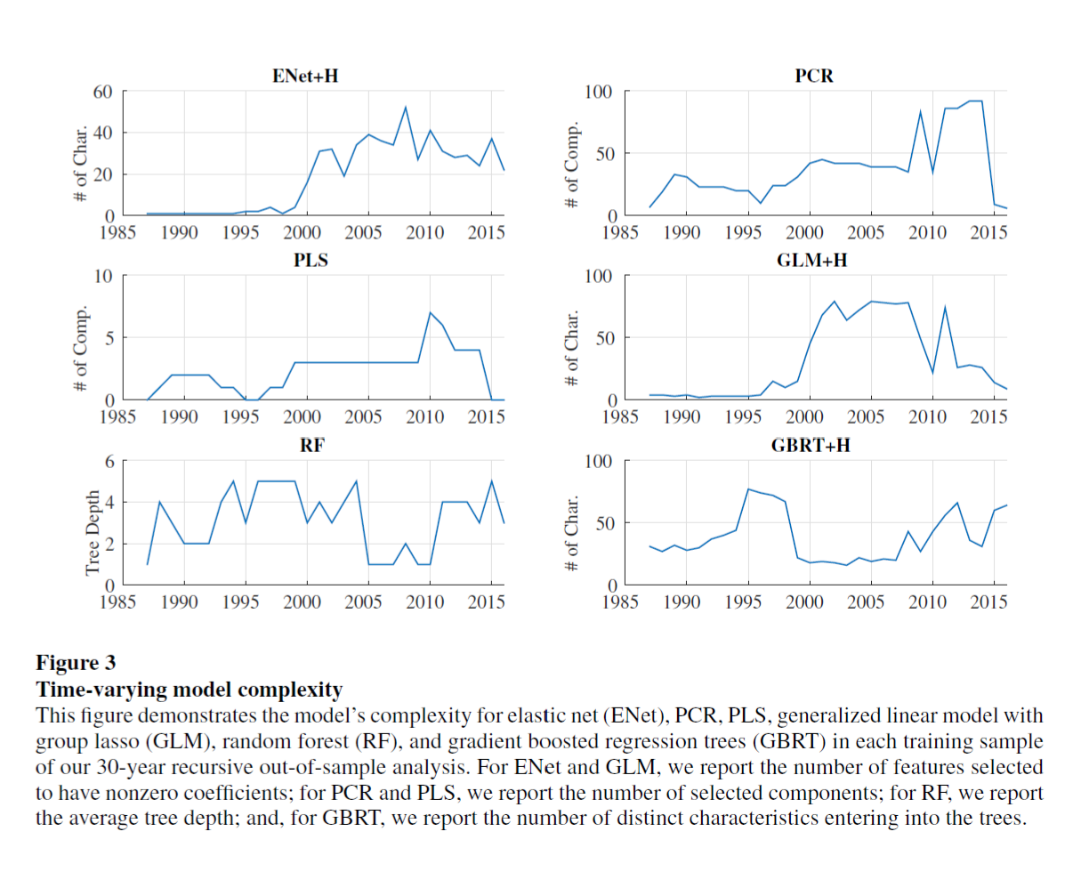
The model complexity has been changing constently, but the measure of the complexity is varying from different model. For example, they choose number of characteristics for Elastic Net and Generalized Linear model, choose number of components for PCR and Partial Linear Square, and choose average tree depth for Gradient Boosted Regression Tree.

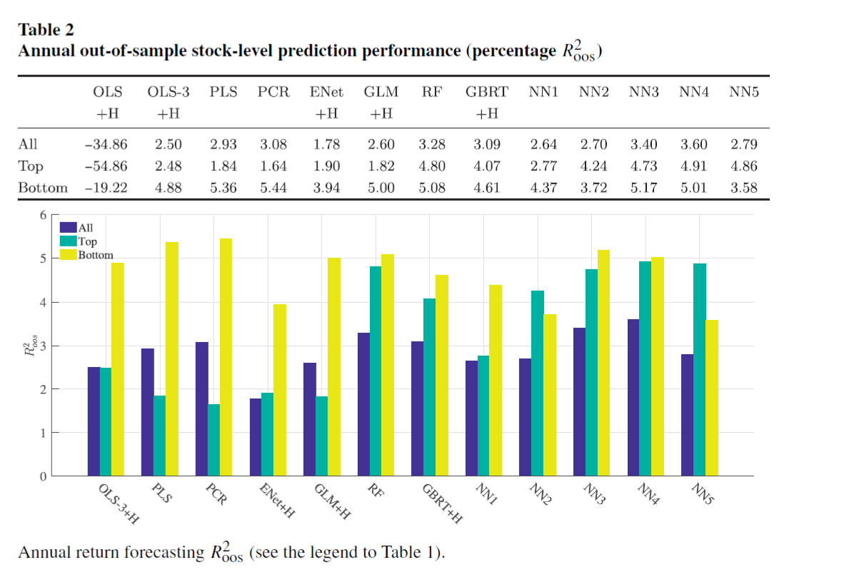
The annual horizon analysis shows a larger magnitude of $R^2$, which indicating ML methods are able to isolate risk premiums that persist over business cycle frequencies and are not merely capturing short-lived inefficiencies.

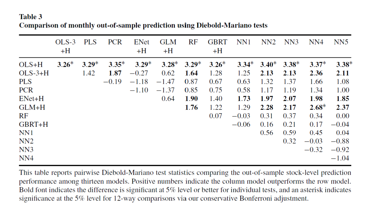
This table shows the statistical significance of differences among models at the monthly frequncy. The Diebold-Mariano statistics are distributed $\matbb N(0,1)$ under the null no difference. The positive values in the NN3 column showing that NN3 out perform all other models.

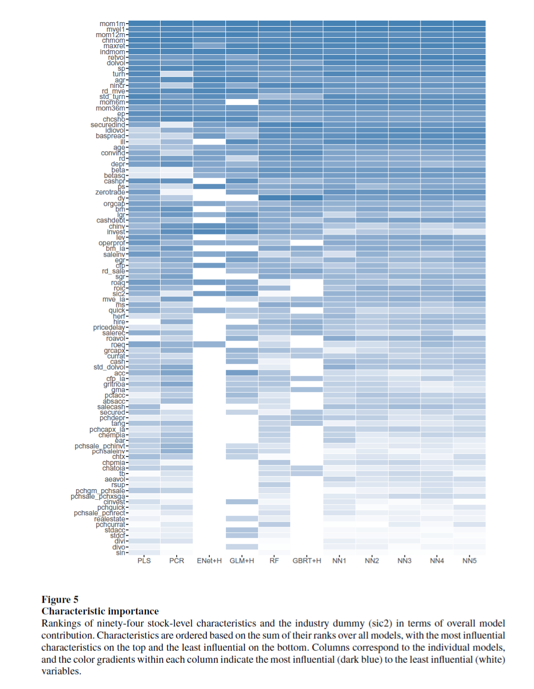
2.3 Which covariates matters

2.4 Portfolio forecast

They build bottom-up forecasts by aggregating individual stock return into portfolios, $w^p_{i,t}$ is the weight of stock i in portfolio p: \(\hat r^p_{t+1} = \sum^n_{i=t}w^p_{i,t} \times \hat r_{i,t+1}\)

Translate $R^2$ into sharp ratio, which matters for mean-variance investors: \(SR^{\ast} = \sqrt \frac{SR^2 + R^2}{1-R^2}\)

and the table below shows the improvement of sharp ratio by the using machine learning methods, which is simply $(SR^{\ast} - SR)$

Cumulative return of machine learning portfolios: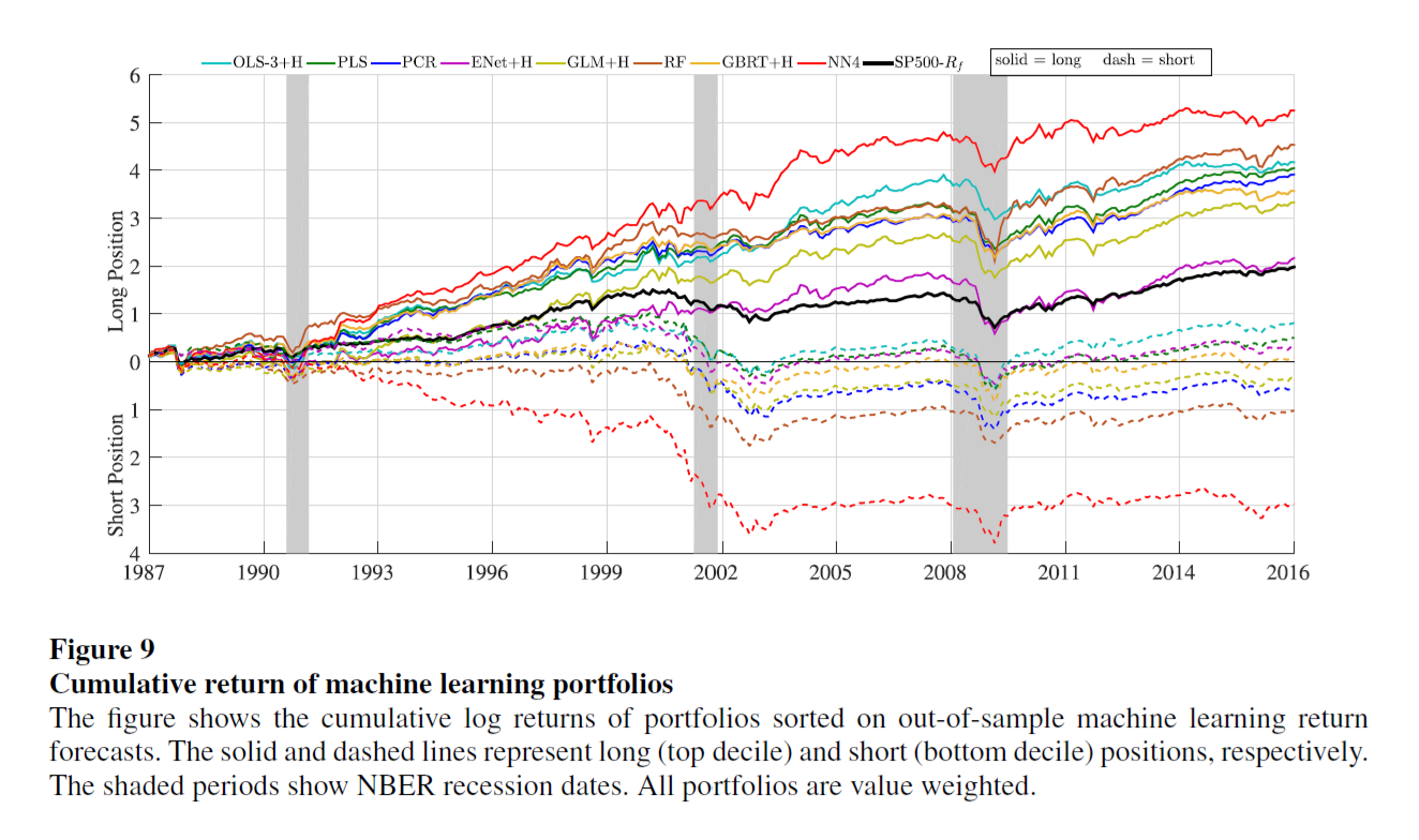

3 Conclusion

This paper uses a widely studied topic – predicting returns as a playground, testing different kinds of machine learning methods, the result shows that machine learning can help improve predicting ability for asset returns. Most importantly this paper stands for a standard machine learning text book help new researchers and practitioners understand the mystery of those methods in fin tech industry.